1 비구획 분석이란
1.1 이 장에서는
약동학과 비구획 분석에 대해 간략히 알아보겠습니다.
1.2 약동학
인체에 약물이 들어올 때, 약물의 양과 효과는 관련성이 있습니다. 따라서 약물의 효과를 파악하기 위해 우리 몸에서 약물이 가지는 약동학적 특성을 파악하는 것은 중요합니다. 다양한 신약 개발 과정에서 이러한 약동학적 특성을 파악하여, 약물의 개발을 지속하거나 중지하기도 하며, 마취통증의학과나 내과 등의 다양한 임상 의학에서도 신체에 중요 영향을 미칠 수 있는 약물에 대하여 대략적인 농도를 파악하기 위해 약물의 약동학적 특성을 이용합니다.
약동학적 약물의 특성은 간단하게 ADME라는 용어로 설명할 수 있습니다. 이는 absorption (흡수), distribution (분포), metabolism (대사), excretion (배설)을 의미합니다. 약물이 다양한 경로 (경구제 복용, 피하 주사, 정맥 주사, 근육 주사 등)를 통해 우리 몸에 들어오게 되면, 정맥주사 이외의 나머지는 흡수 (absorption)의 과정을 거쳐 우리 몸의 정맥에 분포하게 되며, 이러한 약물은 분포 (distribution)와 제거 (metabolism) 과정에서 감소하게 되고, 제거 과정은 우리 몸에 투여된 물질이 여러 기관 (organ)을 통해서 다른 물질로 변하여 (metabolism) 제거되거나 물질이 변화하지 않고 그대로 배설 (excretion) 되는 과정으로 진행되게 됩니다. 이러한 수치들은 각각 약물의 농도가 증가하고 감소하는 과정과 밀접하게 연관되어 있으며, 이러한 과정들을 정량화하여 식을 세울 수 있다면, 약물을 투여한 이후의 농도를 보다 정확하게 예측할 수 있습니다. 이 때 흡수와 관련된 지표로는 흡수속도 상수 (absorption rate constant)와 생체이용률 (bioavailability), 분포, 제거와 관련된 지표로는 분포용적 (Volume of distribution)과 청소율 (Clearance)을 이용하게 되며, 다음 값들을 정확하게 예측하는 것이 약동학 분야에서의 핵심 중의 하나라고 볼 수 있습니다.
이러한 지표들을 구하기 위해서 현재 여러가지 방법들을 사용하고 있으며, 그 중 가장 간단하고도 객관적이며 널리 쓰이는 방법은 비구획분석 (Non-compartmental analysis, NCA)으로 미국의 FDA (Food and Drug Administration)에서는 NCA 계산을 하는 소프트웨어를 규정하고 있지 않아, 상용 소프트웨어를 사용하지 않고 약동학적 지표를 구하는 것을 허용하고 있습니다. 따라서 무료로 누구나 사용할 수 있는 R 패키지를 사용하여 주어진 시간과 농도로부터 비구획 분석 방법으로 약동학적 주요 지표를 직접 구해보고자 합니다.
1.3 비구획 분석 이론 및 계산 방법
비구획 분석이란 시간, 농도가 표현되어 있는 곡선에서 아무런 가정을 하지 않고 분석하는 것을 의미합니다. 이때 다음과 같은 가정을 통해서 최대농도 (Cmax) 및 최대농도에 도달하는 시간 (Tmax), 전체 시간-농도 곡선의 면적 (Area under the time-concentration curve, AUC)등을 구하게 됩니다. 이를 통해 측정된 지표들을 통하여 약물의 특성을 파악하고 특정구간에서의 농도를 예측하게 됩니다. 비구획 분석에서는 statistical moment theory (단순히 하나의 분자가 우리 몸에 들어와서 제거되지 까지는 예측하는 것이 힘들지만 그 개개의 분자들의 양이 늘어날수록 그들의 전반적인 행동이 규칙적으로 이루어진다는 이론)를 가정하고 이를 통해 우리는 각각의 분자가 우리 몸에서 얼마나 머무는지에 대한 평균값을 예상할 수 있게 됩니다. 이 시간을 MRT (mean residence time)이라고 지칭하게 되며, 이것은 농도와 시간의 곱을 적분한 값에서 단순 농도 값을 적분한 농도를 나누어 준 값으로 다음과 같이 표현해 줄 수 있습니다. (Equation (1.1)) \[\begin{equation} MRT = \frac{AUMC}{AUC} = \frac{\int_{0}^{\infty} t \cdot C(t) dt}{\int_{0}^{\infty} C(t) dt} \tag{1.1} \end{equation}\]
이때 식에서 표현된 AUMC는 area under the first moment curve로 농도와 시간의 곱을 시간에 대해서 적분한 값에 해당하며 AUC는 area under concentration으로 농도를 시간에 대해 적분한 값에 해당합니다. 하지만 이 때, 각각의 약물에서 농도와 시간 사이의 명확한 함수관계를 확인할 수 없고, 주어진 정보도 제한적이므로 농도를 시간으로 적분하기에는 상당한 어려움이 따릅니다. 따라서 이를 간소화 하기 위해 Linear trapezoidal method(농도-시간 곡선에서 농도를 측정한 점과 점 사이의 면적을 사다리꼴이라 가정하고 넓이를 구하는 방식)를 사용하게 됩니다. 처음 농도를 측정한 부분부터 마지막 샘플까지를 t1,t2 …tlast로 표현했을 시 t1과 t2의 사이의 AUC와 AUMC는 다음과 같이 계산됩니다.1 \[\begin{equation} \begin{split} AUC_{t_1-t_2} & = (t_2-t_1)\cdot \frac{C_2+C_1}{2} \\ AUMC_{t_1-t_2} & = (t_2-t_1)\cdot \frac{t_2 \cdot C_2 + t_1 \cdot C_1}{2} \end{split} \tag{1.2} \end{equation}\]
이 방식을 계속 이용하여 각각의 구간 값의 합을 모두 더한 값으로 AUClast(처음 농도를 측정하기 시작한 구간부터 마지막 농도를 측정한 구간까지 linear trapezoidal method를 통해서 값을 계산한 방식), AUMClast(처음 농도를 측정하기 시작한 구간부터 마지막 농도를 측정한 구간까지 linear trapezoidal method를 통해서 값을 계산한 방식)를 측정해 주게 됩니다. (그림 1.1)
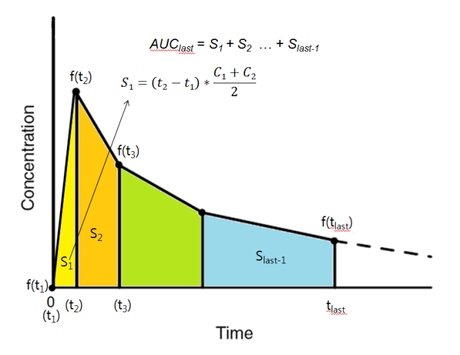
Figure 1.1: Linear trapezoidal method
추가적으로 마지막으로 농도를 잰 시점에서 모든 약물이 우리 몸에서 빠져나가는 시점까지의 값을 구하기 위해서 마지막으로 측정한 점의 기울기가 그대로 약물이 모두 제거되는 시점까지 그대로 유지된다는 가정을 세우게 됩니다. 다음과 같이 Clast(가장 마지막으로 농도를 측정한 시점)에서 λ (Cmax 이후에 선형성이 가장 높은 3점을 선택하여 구한 기울기)를 구한 후 다음과 같은 약동학 공식을 대입하여 값을 구해주게 됩니다. \[\begin{equation} \begin{split} AUC_{t_{last}-\infty} = \frac{C_{last}}{\lambda} \\ AUMC_{t_{last}-\infty} = \frac{t_{last} \cdot C_{last}}{\lambda} + \frac{C_{last}}{\lambda^2} \end{split} \tag{1.3} \end{equation}\]
약물이 우리 몸에 들어온 후 가장 높은 농도의 경우 실제 개개인에서 농도를 측정한 값들 중 가장 높은 농도를 실제 가장 높은 농도라 가정하여 사용하게 되고, 이 지표를 Cmax라 부릅니다. 또한 이때의 시점을 Tmax라 부르게 됩니다. 위에서 구한 AUC와 Cmax, λ 를 가지고 나머지 주요 값을 계산하게 됩니다. 이 중 청소율(제거되는 속도)에 해당하는 clearance(일반적으로 CL이라 지칭한다.) 의 경우 다음의 약동학 기본 공식을 활용하여 구해주게 됩니다. \[\begin{equation} CL = \frac{D \cdot F}{AUC} \tag{1.4} \end{equation}\]
수식에서 D는 dose로 투여량을, F는 생체이용률을 의미합니다.
우리 몸의 분포 (disposition)을 알기 위해 우리 몸의 volume을 나타내는 volume of distribution at steady state (Vdss)는 아래 식을 이용하여 값을 구하게 됩니다.
\[ Vd_{ss} = MRT \cdot CL = \frac{AUMC}{AUC} \cdot \frac{D}{AUC} \]
우리 몸의 생체이용률을 나타내는 F의 경우 기본적으로 정맥주사시의 생체이용률을 1이라고 가정하고, 다음 식으로 구합니다.
\[ F = \frac{D_{iv}}{D_{oral}} \cdot \frac{AUC_{oral}}{AUC_{iv}} \]
(이중 Div는 정맥주사 투여량, Doral은 경구 투여량, AUCoral은 경구 투여에서의 AUC, AUCiv는 정맥투여에서의 AUC를 의미한다. 이처럼 AUC, Cmax, AUMC, λ 를 구하는 부분에 있어서는 non-compartmental analysis의 기본 가정들을 활용하였고 그 밖의 부분들에서는 현재 정형화된 공식들을 활용하여 적용하였다. 위 내용을 바탕으로 R을 기반으로 한 script를 구성한 후 전세계적으로 널리 쓰이고 있는 CDISC terminology를 각각의 지표들에 적용하여 결과값을 도출하였다.
또한 투여되는 방식을 3가지 분류(Extravascular, IV infusion, IV bolus)로 구분하여, 그에 맞는 각각의 식을 적용하였다. 마지막으로 시간당 농도의 변화율이 농도 증가 곡선보다 감소 곡선에서 완만하다는 점을 고려하여 농도가 감소하는 구간에서는 log값을 선택적으로 줄 수 있도록 설정하였으며, 흡수 속도 상수의 경우 현 NCA method를 통해 구하기에는 한계가 있어 따로 값을 제시하지 않았습니다.
흡수속도 상수를 구하기 위해서는 구획분석방법(compartmental analysis)이나 비선형 혼합모형(non-linear mixed effect modeling)을 사용하는 것이 바람직합니다.
Figure 2. Linear trapezoidal method를 적용한 AUC의 계산 Script
Figure 3 약동학 지표들에 대해 각각의 공식을 적용한 Script의 예
1.4 계산 공식
C0: C0 is the initial concentration at the dosing time. It is the observed concentration at the dosing time, if available. Otherwise it is approximated using the following rules. For iv-bolus data, log-linear back-extrapolation (see “backExtrap” argument) is performed from the first two observations to estimate C0, provided the local slope is negative. However, if the slope is >=0 or at least one of the first two concentrations is 0, the first non-zero concentration is used as C0. For other types of administration, C0 is equal to 0 for non steady-state data and for steady-state data the minimum value observed between the dosing intervals is used to estimate C0, provided the “backExtrap” argument is set to “yes”.
Cmax, Tmax and Cmax_D: Cmax and Tmax are the value and the time of maximum observed concentration, respectively. If the maximum concentration is not unique, the first maximum is used. For steady state data, The maximum value between the dosing intervals is considered. Cmax_D is the dose normalized maximum observed concentration.
Clast and Tlast
Clast and Tlast are the last measurable positive concentration and the corresponding time, respectively.
AUClast
The area under the concentration vs. time curve from the first observed to last measurable concentration.
AUMClast
The area under the first moment of the concentration vs. time curve from the first observed to last measurable concentration.
MRTlast
Mean residence time from the first observed to last measurable concentration. For non-infusion models,
\(MRTlast = \frac{AUMClast}{AUClast}\)
For infusion models,
\(MRTlast = \frac{AUMClast}{AUClast}-\frac{TI}{2}\)
where TI is the infusion duration.
No_points_Lambda_z
No_points_Lambda_z is the number of observed data points used to determine the best fitting regression line in the elimination phase.
AUC_pBack_Ext_obs and AUC_pBack_Ext_pred
The percentage of AUC that is contributed by the back extrapolation to estimate C0. The rules to to estimate C0 is given above.
AUClower_upper
The AUC under the concentration-time profile within the user-specified window of time provided as the “AUCTimeRange” argument. In case of empty “AUCTimeRange” argument, AUClower_upper is equal to the AUClast.
Rsq, Rsq_adjusted and Corr_XY
Regression coefficient of the regression line used to estimate the elimination rate constant. Rsq_adjusted is the adjusted value of Rsq given by the following relation.
\(Rsq\_adjusted = 1-\frac{(1-Rsq^2)*(n-1)}{n-2}\)
where n is the number of points in the regression line. Corr_XY is the square root of Rsq.
Lambda_z
Elimination rate constant estimated from the regression line representing the terminal phase of the concentration-time profile. The relation between the slope of the regression line and Lambda_z is:
\(Lambda\_z = -(slope)\)
Lambda_lower and Lambda_upper
Lower and upper limit of the time values from the concentration-time profile used to estimate Lambda_z, respectively, in case the “LambdaTimeRange” is used to specify the time range.
HL_Lambda_z
Terminal half-life of the drug:
\(HL\_Lambda\_z = \frac{ln2}{\lambda_z}\)
AUCINF_obs and AUCINF_obs_D
AUC estimated from the first sampled data extrapolated to \({\infty}\). The extrapolation in the terminal phase is based on the last observed concentration (\({Clast_obs}\)). The equation used for the estimation is given below.
\(AUCINF\_obs = AUClast+\frac{Clast\_obs}{\lambda_z}\)
AUCINF_obs_D is the dose normalized AUCINF_obs.
AUC_pExtrap_obs
Percentage of the AUCINF_obs that is contributed by the extrapolation from the last sampling time to \({\infty}\).
\(AUC\_pExtrap\_obs = \frac{AUCINF\_obs-AUClast}{AUCINF\_obs}*100\%\)
AUMCINF_obs
AUMC estimated from the first sampled data extrapolated to \({\infty}\). The extrapolation in the terminal phase is based on the last observed concentration. The equation used for the estimation is given below.
\(AUMCINF\_obs = AUMClast+\frac{Tlast*Clast\_obs}{\lambda_z}+\frac{Clast\_obs}{\lambda_{z}^2}\)
AUMC_pExtrap_obs
Percentage of the AUMCINF_obs that is contributed by the extrapolation from the last sampling time to \({\infty}\).
\(AUMC\_pExtrap\_obs = \frac{AUMCINF\_obs-AUMClast}{AUMCINF\_obs}*100\%\)
Vz_obs
Volume of distribution estimated based on total AUC using the following equation.
\(Vz\_obs = \frac{Dose}{\lambda_z*AUCINF\_obs}\)
Cl_obs
Total body clearance.
\(Cl\_obs = \frac{Dose}{AUCINF\_obs}\)
AUCINF_pred and AUCINF_pred_D
AUC from the first sampled data extrapolated to \({\infty}\). The extrapolation in the terminal phase is based on the last predicted concentration obtained from the regression line used to estimate Lambda_z (\({Clast\_pred}\)). The equation used for the estimation is given below.
\(AUCINF\_pred = AUClast+\frac{Clast\_pred}{\lambda_z}\)
AUCINF_pred_D is the dose normalized AUCINF_pred.
AUC_pExtrap_pred
Percentage of the AUCINF_pred that is contributed by the extrapolation from the last sampling time to \({\infty}\).
\(AUC\_pExtrap\_pred = \frac{AUCINF\_pred-AUClast}{AUCINF\_pred}*100\%\)
AUMCINF_pred
AUMC estimated from the first sampled data extrapolated to \({\infty}\). The extrapolation in the terminal phase is based on the last predicted concentration obtained from the regression line used to estimate Lambda_z (\({Clast\_pred}\)). The equation used for the estimation is given below.
\(AUMCINF\_pred = AUMClast+\frac{Tlast*Clast\_pred}{\lambda_z}+\frac{Clast\_pred}{\lambda_{z}^2}\)
AUMC_pExtrap_pred
Percentage of the AUMCINF_pred that is contributed by the extrapolation from the last sampling time to \({\infty}\).
\(AUMC\_pExtrap\_pred = \frac{AUMCINF\_pred-AUMClast}{AUMCINF\_pred}*100\%\)
Vz_pred
Volume of distribution estimated based on total AUC using the following equation.
\(Vz\_pred = \frac{Dose}{\lambda_z*AUCINF\_pred}\)
Cl_pred
Total body clearance.
\(Cl\_pred = \frac{Dose}{AUCINF\_pred}\)
MRTINF_obs
Mean residence time from the first sampled time extrapolated to \({\infty}\) based on the last observed concentration (\({Clast\_obs}\)).
For non-infusion non steady-state data:
\(MRTINF\_obs = \frac{AUMCINF\_obs}{AUCINF\_obs}\)
For infusion non steady-state data:
\(MRTINF\_obs = \frac{AUMCINF\_obs}{AUCINF\_obs}-\frac{TI}{2}\)
where \({TI}\) is the infusion duration. For non-infusion steady-state data:
\(MRTINF\_obs = \frac{AUMCINF\_obs|_{0}^{\tau}+\tau*(AUCINF\_obs-AUC|_{0}^{\tau})}{AUCINF\_obs|_{0}^{\tau}}\)
For infusion steady-state data:
\(MRTINF\_obs = \frac{AUMCINF\_obs|_{0}^{\tau}+\tau*(AUCINF\_obs-AUC|_{0}^{\tau})}{AUCINF\_obs|_{0}^{\tau}}-\frac{TI}{2}\)
For steady-state data \({\tau}\) represents the dosing interval.
MRTINF_pred
Mean residence time from the first sampled time extrapolated to \({\infty}\) based on the last predicted concentration obtained from the regression line used to estimate Lambda_z (\({Clast\_pred}\)).
For non-infusion non steady-state data:
\(MRTINF\_pred = \frac{AUMCINF\_pred}{AUCINF\_pred}\)
For infusion non steady-state data:
\(MRTINF\_pred = \frac{AUMCINF\_pred}{AUCINF\_pred}-\frac{TI}{2}\)
where \({TI}\) is the infusion duration.
For non-infusion steady-state data:
\(MRTINF\_pred = \frac{AUMCINF\_pred|_{0}^{\tau}+\tau*(AUCINF\_pred-AUC|_{0}^{\tau})}{AUCINF\_pred|_{0}^{\tau}}\)
For infusion steady-state data:
\(MRTINF\_pred = \frac{AUMCINF\_pred|_{0}^{\tau}+\tau*(AUCINF\_pred-AUC|_{0}^{\tau})}{AUCINF\_pred|_{0}^{\tau}}-\frac{TI}{2}\)
For steady-state data \({\tau}\) represents the dosing interval.
Vss_obs and Vss_pred
An estimate of the volume of distribution at steady-state.
\(Vss\_obs = MRTINF\_obs*Cl\_obs\)
\(Vss\_pred = MRTINF\_pred*Cl\_pred\)
Tau
The dosing interval for steady-state data. This value is assumed to be the same over multiple doses.
Cmin and Tmin
Cmin is the minimum concentration between 0 and Tau and Tmin is the corresponding time for steady-state data.
Cavg
The average concentration between 0 and Tau for steady-state data.
\(Cavg = \frac{AUC|_{0}^{Tau}}{Tau}\)
p_Fluctuation
Percentage of the fluctuation of the concentration between 0 and Tau for steady-state data.
\(p\_Fluctuation = \frac{Cmax-Cmin}{Cavg}*100\%\)
Accumulation_Index
\(Accumulation\_Index = \frac{1}{1-e^{-\lambda_{z}*\tau}}\)
Clss
An estimate of the total body clearance for steady-state data.
\(Clss = \frac{Dose}{AUC|_{0}^{\tau}}\)
참고문헌
Bae, Kyun-Seop. 2019. Ncar: Noncompartmental Analysis for Pharmacokinetic Report. https://CRAN.R-project.org/package=ncar.
Bae, Kyun-Seop. 2020. NonCompart: Noncompartmental Analysis for Pharmacokinetic Data. https://CRAN.R-project.org/package=NonCompart.
Bae, Kyun-Seop, and Jee Eun Lee. 2018. Pkr: Pharmacokinetics in R. https://CRAN.R-project.org/package=pkr.
이 수식은
NonCompart::AUC()함수에서 계산 되게 됩니다.↩︎