caffsim R package: Simulation of Plasma Caffeine Concentrations by Using Population Pharmacokinetic Model
![]()
Simulate plasma caffeine concentrations using population pharmacokinetic model described in Lee, Kim, Perera, McLachlan and Bae (2015) doi:10.1007/s00431-015-2581-x and the package was published doi:10.12793/tcp.2017.25.3.141.
- Github: https://github.com/asancpt/caffsim
- Package vignettes and references by
pkgdown: http://asancpt.github.io/caffsim
Installation
install.pacakges("devtools")
devtools::install_github("asancpt/caffsim")

# Simply create single dose dataset
caffsim::caffPkparam(Weight = 20, Dose = 200, N = 20)

# Simply create multiple dose dataset
caffsim::caffPkparamMulti(Weight = 20, Dose = 200, N = 20, Tau = 12)
Single dose
Create a PK dataset for caffeine single dose
library(caffsim)
MyDataset <- caffPkparam(Weight = 20, Dose = 200, N = 20)
head(MyDataset)
## # A tibble: 6 x 9
## subjid Tmax Cmax AUC Half_life CL V Ka Ke
## <int> <dbl> <dbl> <dbl> <dbl> <dbl> <dbl> <dbl> <dbl>
## 1 1 0.183 16.1 191. 8.07 1.05 12.2 32.5 0.0858
## 2 2 0.532 11.2 82.8 4.75 2.41 16.6 7.58 0.146
## 3 3 2.36 10.2 150. 8.33 1.34 16.1 1.22 0.0832
## 4 4 0.731 10.5 62.8 3.60 3.19 16.6 4.51 0.192
## 5 5 0.599 12.9 62.0 2.89 3.23 13.4 5.46 0.240
## 6 6 1.08 12.4 104. 5.01 1.92 13.9 2.99 0.138Create a dataset for concentration-time curve
MyConcTime <- caffConcTime(Weight = 20, Dose = 200, N = 20)
head(MyConcTime)
## # A tibble: 6 x 3
## Subject Time Conc
## <dbl> <dbl> <dbl>
## 1 1 0 0
## 2 1 0.1 6.46
## 3 1 0.2 10.2
## 4 1 0.3 12.4
## 5 1 0.4 13.5
## 6 1 0.5 14.1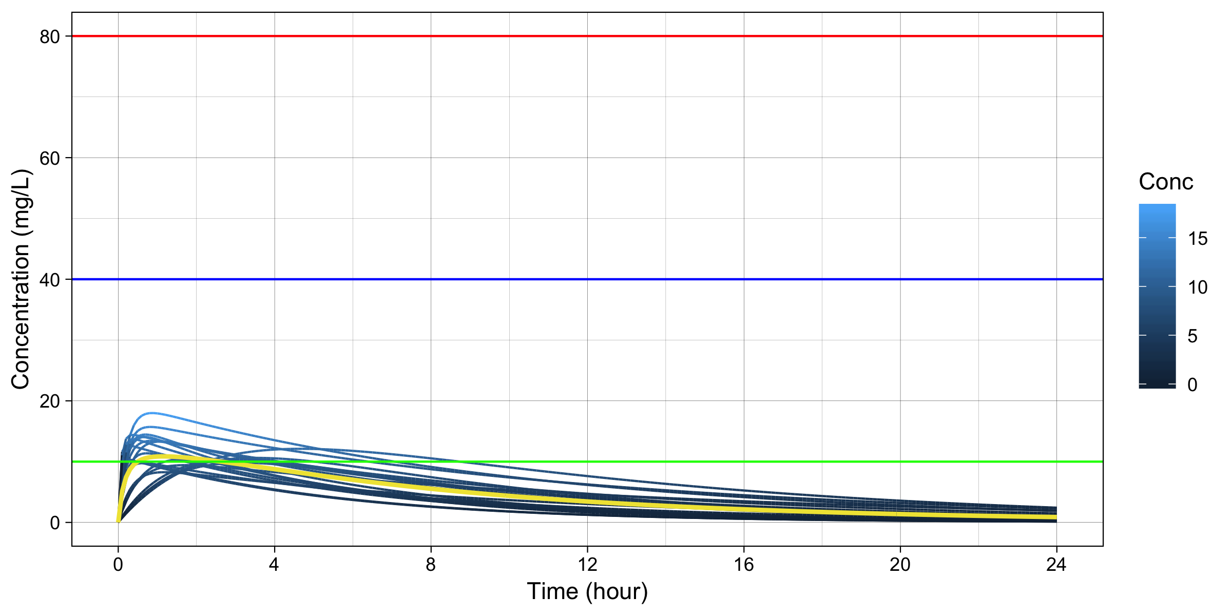
Create plots for publication (according to the amount of caffeine)
-
cowplotpackage is required
#install.packages("cowplot") # if you don't have it
library(cowplot)

MyPlotPub <- lapply(
  c(seq(100, 800, by = 100)),
  function(x) caffPlotMulti(caffConcTime(20, x, 20)) +
    theme(legend.position="none") +
    labs(title = paste0("Single Dose ", x, "mg")))

plot_grid(MyPlotPub[[1]], MyPlotPub[[2]],
          MyPlotPub[[3]], MyPlotPub[[4]],
          MyPlotPub[[5]], MyPlotPub[[6]],
          MyPlotPub[[7]], MyPlotPub[[8]],
          labels=LETTERS[1:8], ncol = 2, nrow = 4)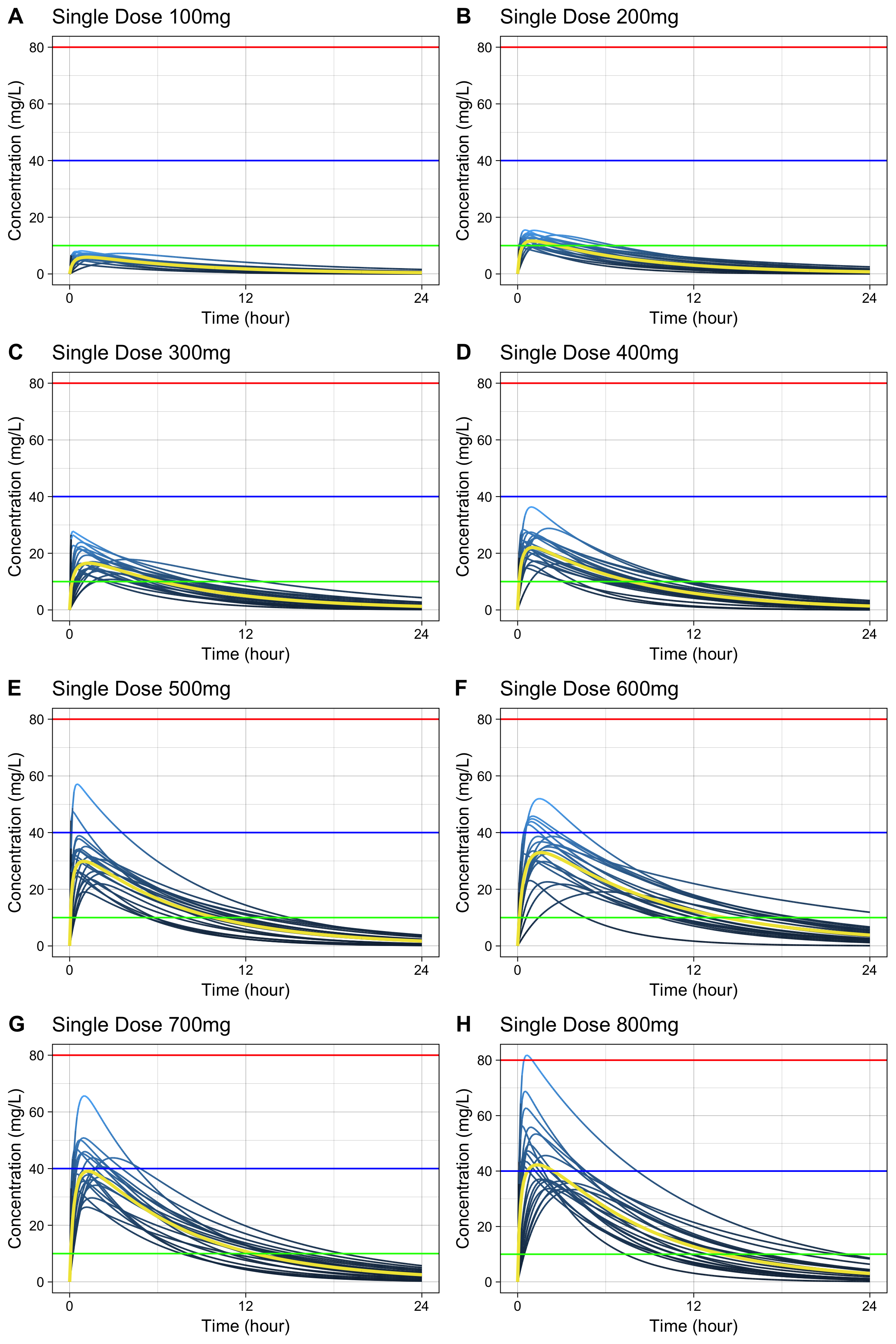
Multiple dose
Create a PK dataset for caffeine multiple doses
MyDatasetMulti <- caffPkparamMulti(Weight = 20, Dose = 200, N = 20, Tau = 12)
head(MyDatasetMulti)
## # A tibble: 6 x 9
## subjid TmaxS CmaxS AUCS AI Aavss Cavss Cmaxss Cminss
## <int> <dbl> <dbl> <dbl> <dbl> <dbl> <dbl> <dbl> <dbl>
## 1 1 1.20 10.2 75.9 1.16 102. 6.32 14.4 2.04
## 2 2 2.56 12.0 165. 1.50 181. 13.7 22.7 7.51
## 3 3 0.193 15.0 105. 1.21 114. 8.75 18.6 3.21
## 4 4 1.04 12.9 86.0 1.13 92.1 7.17 17.5 2.01
## 5 5 1.10 13.9 114. 1.22 116. 9.51 19.9 3.58
## 6 6 0.804 12.9 103. 1.23 119. 8.62 17.8 3.33Create a dataset for concentration-time curve
MyConcTimeMulti <- caffConcTimeMulti(Weight = 20, Dose = 200, N = 20, Tau = 12, Repeat = 10)
head(MyConcTimeMulti)
## # A tibble: 6 x 3
## # Groups: Subject [1]
## Subject Time Conc
## <dbl> <dbl> <dbl>
## 1 1 0 0
## 2 1 0.1 6.76
## 3 1 0.2 10.8
## 4 1 0.3 13.1
## 5 1 0.4 14.5
## 6 1 0.5 15.2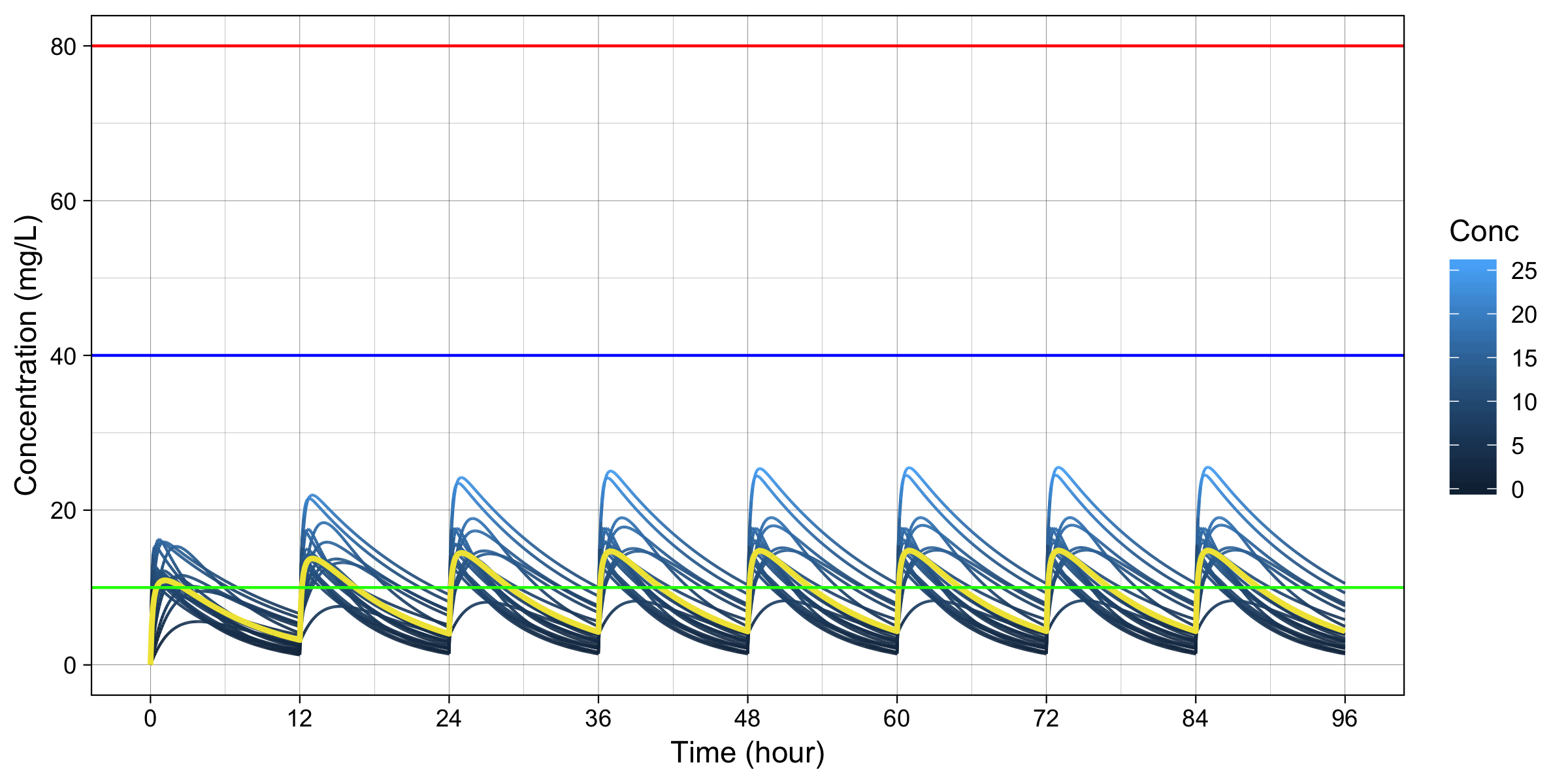
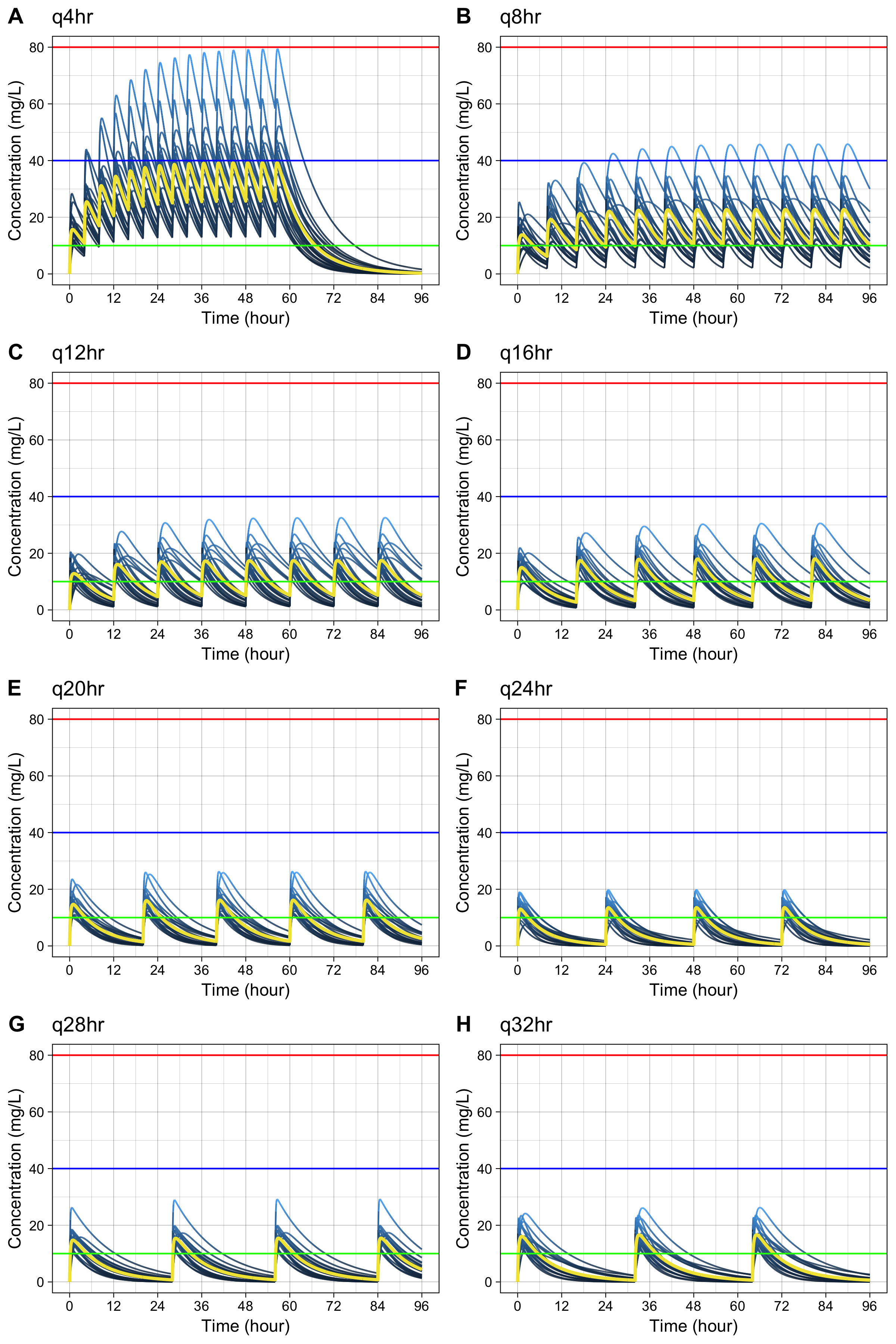
Create plots for publication (according to dosing interval)
-
cowplotpackage is required
#install.packages("cowplot") # if you don't have it
library(cowplot)

MyPlotMultiPub <- lapply(
  c(seq(4, 32, by = 4)),
  function(x) caffPlotMulti(caffConcTimeMulti(20, 250, 20, x, 15)) +
    theme(legend.position="none") +
    labs(title = paste0("q", x, "hr" )))

plot_grid(MyPlotMultiPub[[1]], MyPlotMultiPub[[2]],
          MyPlotMultiPub[[3]], MyPlotMultiPub[[4]],
          MyPlotMultiPub[[5]], MyPlotMultiPub[[6]],
          MyPlotMultiPub[[7]], MyPlotMultiPub[[8]],
          labels=LETTERS[1:8], ncol = 2, nrow = 4)